Porting a model from NEURON to PyNN: a case study
Tags: reproducible research, Python, NEURONPorting a model from a simulator-specific format to PyNN allows the model to be simulated on other simulators (for cross-checking or for inclusion as a component in a larger model) or on neuromorphic hardware.
This article documents the process of converting one of the models described in Destexhe (2009) (preprint), originally written in Hoc for the NEURON simulator, to Python, using the PyNN API.
In summary, the process is:
- convert the code from Hoc to Python, which is fairly straightforward due to the similarities in syntax;
- one at a time, replace the original NMODL mechanisms with the nearest equivalent mechanisms provided by PyNN;
- incrementally replace NEURON-specific Python code with the equivalent from PyNN.
- after each incremental step, run the simulation and check that the results are qualitatively unchanged (sometimes they should be quantitatively unchanged as well, but sometimes, as when changing random number generators for example, this is not achievable).
For more details, read on.
If you would like to follow along and run the code on your own machine, all of the code is in a Mercurial repository at https://bitbucket.org/apdavison/destexhe_jcns_2009, and each change to the code has been saved to the repository as a separate commit. To get started:
$ hg clone https://bitbucket.org/apdavison/destexhe_jcns_2009
$ cd destexhe_jcns_2009
$ hg update -r 0         # work with the initial version of the code
The original implementation
$ cd demo_cx-lts
$ ls
IF_BG4.mod          demo_cx05_N=500b_LTS.oc multiAMPAexp.mod        multiStimexp.mod
README              gen5.mod                multiGABAAexp.mod
These are the files that Alain Destexhe originally sent me. You can see that we have one Hoc file and a bunch of NMODL files. The model is a cortical network consisting of 500 excitatory and inhibitory cells, in the proportion 4:1, and random connectivity. The excitatory cells include a proportion of LTS (low-threshold spiking) cells. All cells are modelled as Brette-Gerstner adapative exponential integrate-and-fire neurons, implemented by the IF_BG4.mod mechanism.
Neurons are implemented by a template CXcell, which creates a single compartment and inserts the pas and IF_BG4 mechanisms. The network is built through a series of procedures: netCreate(), netConnect() and insertStimulation(). The simulation is run through procedure run_sim(), which calls the standard neuron init() and run() procedures, then writes spikes for all cells and the membrane potential for a single cell to file.
netCreate() loops over excitatory cells, each time creating a CXcell and storing it in an array neuron[N_CX], setting RS (regular spiking) parameters, drawing a random number in [0,1] to determine whether the cell is an LTS cell, in which case some of the parameters are changed, and creating synapses by calling the procedures setExpAMPA(), setExpGABA(), setExpStim(). It then loops over inhibitory cells, creating more CXcell objects, setting FS (fast spiking) parameters and creating synapses.
netConnect() has an outer loop over all post-synaptic cells, which contains a loop over excitatory pre-synaptic cells followed by a loop over inhibitory pre-synaptic cells. Within each loop, a random number in [0,1] is drawn and used to determine whether each possible connection is made or not, based on a connection probability PROB_CONNECT. If a connection is to be made, the method addlink() of the corresponding synapse object neuron[i].ampa or neuron[i].gaba is called with a reference to the membrane potential of the pre-synaptic neuron. This creates a pointer from the synapse mechanism to the pre-synaptic membrane potential. The inner loops are exited prematurely if the number of connections created passes a threshold. This means that on multiple runs of the network with different random seeds, the number of connections will follow a truncated binomial distribution.
insertStimulation() loops over a subset of the neurons (since they are ordered by type, it is always the excitatory neurons that are excited), creates a new gen object (defined in the file gen5.mod), which is a Poisson spike train generator, and connects it to the neuron via an exponential synapse.
Although each synapse type has its own mechanism, multiAMPAexp, multiGABAAexp and multiStimexp, they are essentially identical models, differing only in their parameters. The reason for making them separate mechanisms is to allow global variables to be used for some of the parameters, which is presumably more efficient than using range variables.
Spikes are recorded/stored inside the IF_BG4 mechanism. The membrane potential for the single neuron that is recorded is stored in a global Vector object, Vm.
So, let's compile the NMODL mechanisms and run the simulation (I'm assuming that you're familiar with NEURON and have it installed on your machine. If not, see the NEURON website):
$ nrnivmodl
$ nrngui demo_cx05_N=500b_LTS.oc
This produces three data files: spiketimes_cx05_LTS500b.dat, numspikes_cx05_LTS500b.dat and Vm170_cx05_LTS500b.dat. Note that subsequent runs will overwrite the filenames each time, so be sure to copy the output data files to some uniquely-named directory after each run to avoid this.
The data files I obtained are available by clicking on this
icon: ![]() , which takes you to a record of the precise
environment used to run the simulation (NEURON version, operating system,
processor architecture, etc.) If you have trouble reproducing any of the
results in this article, comparing your own environment to the one I used may
help to identify the cause of the problem. There is a similar icon for each of
the simulations in this article, and clicking on any figure will take you to a
similar record. The environment information was captured automatically using Sumatra.
, which takes you to a record of the precise
environment used to run the simulation (NEURON version, operating system,
processor architecture, etc.) If you have trouble reproducing any of the
results in this article, comparing your own environment to the one I used may
help to identify the cause of the problem. There is a similar icon for each of
the simulations in this article, and clicking on any figure will take you to a
similar record. The environment information was captured automatically using Sumatra.
Plotting the results
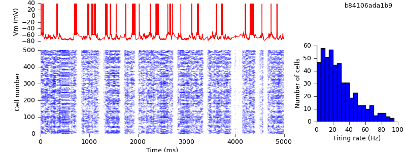
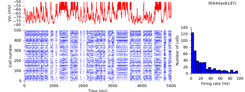
Alain didn't include any plotting code, so I wrote a short Matplotlib script to reproduce a fascimile of Figure 7 from Destexhe (2009):
$ hg update -r 1   # this version adds the plotting script
$ python plot.py spiketimes_cx05_LTS500b.dat numspikes_cx05_LTS500b.dat Vm170_cx05_LTS500b.dat
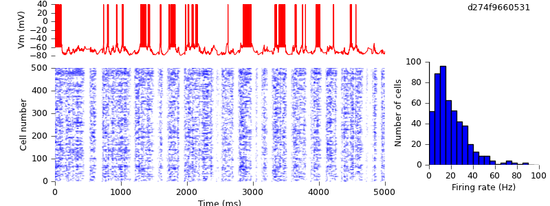
You can see that it is not quantitatively identical to the published figure, but qualitatively shows the same up- and down-state behaviour, with a similar distribution of mean firing rates across the population. The differences are probably due to differences in the sequence of random numbers used to construct the network.
General porting strategy
To port the model from Hoc to PyNN, the approach I have used is the following:
- convert the code from Hoc to Python, which can be done all at once or incrementally, due to the ability to execute fragments of Hoc code from within Python using the h() function (see Hines et al. (2009) for more on this). At each step, we can compare the results to the original output, to check we have changed nothing in the original model.
- incrementally replace the original NMODL mechanisms with the nearest equivalent mechanisms from PyNN, again testing that the output is unchanged. In some cases the nearest PyNN equivalent may be slightly different, as will prove to be the case for the present model, and then we will have to decide whether the output is qualitatively similar enough. In general it is good in any case for the important features of a model not to be too sensitive to the details of individual components.
- incrementally replace NEURON-specific Python code with the PyNN equivalent, testing after each change as in the previous two steps. We will know the conversion is complete when the simulations can be run with both NEST and NEURON.
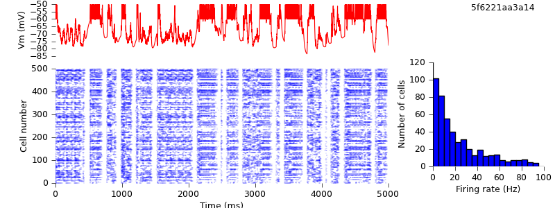
Since it will be important to be able to compare different versions of the code, our first step is to make the original code more reproducible by adding explicit seeds for the random number generators:
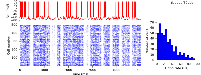
$ hg update -r 2   # this version adds RNG seeds to the Hoc file
$ nrngui demo_cx05_N=500b_LTS.oc
$ python plot.py spiketimes_cx05_LTS500b.dat numspikes_cx05_LTS500b.dat Vm170_cx05_LTS500b.dat
![]()

Because of the different seeds, the results are not quantitatively identical, but the qualitative behaviour of up and down-states is preserved.
Converting from Hoc to Python
The syntax of Hoc and Python is actually fairly similar - most of the changes needed were as simple as replacing the Hoc comment signifier // with #. We keep the names netCreate(), netConnect(), insertSimulation() and run_sim(), which now become Python functions instead of Hoc procedures.
The CXcell template becomes a Python class CXcell, inheriting from nrn.Section to make it a single-compartment NEURON cell (the Python code is quite a bit more concise, which is nice.)
Now we can run the Python version of the code. We would expect to get identical results to the Hoc version.
$ hg update -r 3  # direct translation from Hoc to Python
$ python demo_cx05_N=500b_LTS.py
![]()
And indeed the results are precisely identical.
$ python plot.py spiketimes_cx05_LTS500b.dat numspikes_cx05_LTS500b.dat Vm170_cx05_LTS500b.dat
Replacing the IF_BG4 mechanism with AdExpIF
Now we begin replacing the original NMODL mechanisms with the PyNN equivalent. PyNN has its own implementation of the adaptive exponential integrate-and-fire model for NEURON, called AdExpIF, so the first step is to use that instead of the IF_BG4 mechanism. First we load AdExpIF from wherever we have installed PyNN:
from neuron import load_mechanisms
from pyNN import __path__ as pyNN_path
load_mechanisms(pyNN_path[0] + "/neuron/nmodl")
There are two important differences between IF_BG4 and AdExpIF. The first is that the former is a "density mechanism" while the latter is a "point process", in NEURON terminology. So we replace:
self.soma.insert('IF_BG4')
by:
self.adexp = h.AdExpIF(0.5, sec=self.soma)
Similarly, parameters are set slightly differently, i.e., we replace:
neuron[nbactual].soma.Vtr_IF_BG4 = VTR
with:
neuron[nbactual].adexp.vthresh = VTR
etc. The second important difference is that IF_BG4 also performs recording of spike times, while AdExpIF does not, so we need to add some code at the Python level to do that:
self.spike_times = h.Vector()
self.rec = h.NetCon(self.soma(0.5)._ref_v, None, VTR, 0.0, 0.0, sec=self.soma)
self.rec.record(self.spike_times)
We should also note a small bug in IF_BG4, fortunately one which does not, as we shall see, qualitatively affect the results. The refractory period is implemented by defining a variable reset inside the NMODL function fire(), which is decremented by the integration timestep dt each time fire() is called, i.e. each time the BREAKPOINT block is executed. However, NEURON executes the BREAKPOINT block twice for every timestep, so that reset is reduced twice as fast as intended. This means that when VTR = 5.0, the effective refractory period is actually 2.5 ms.
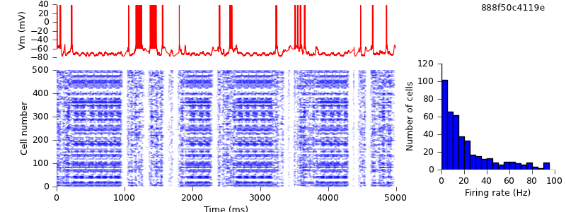
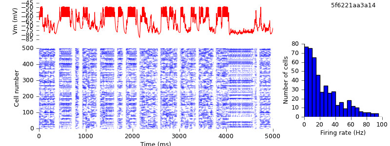
$ hg update -r 4  # replaced IF_BG4 mechanism with AdExpIF
$ python demo_cx05_N=500b_LTS.py
$ python plot.py spiketimes_cx05_LTS500b.dat numspikes_cx05_LTS500b.dat Vm170_cx05_LTS500b.dat
![]()
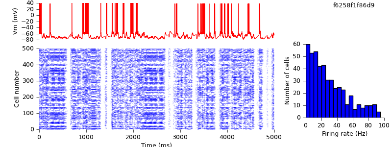
We might have hoped to get quantitatively identical results, but in fact the mean firing rates are slightly higher (33 Hz for RS cells) than in the previous simulation (29 Hz). One source for this difference is the behaviour around threshold. The following table shows part of the data from the Vm170_cx05_LTS500b.dat files for the AdExpIF and IF_BG4 versions, as the membrane potential reaches threshold and is reset.
| t | v (mV) | |
|---|---|---|
| (ms) | AdExpIF | IF_BG4 |
| 6.3 | -52.7427 | -52.7427 |
| 6.4 | -51.9997 | -51.9997 |
| 6.5 | -51.2844 | -51.2844 |
| 6.6 | -50.595 | -50.595 |
| 6.7 | 40 | -49.9297 |
| 6.8 | -60 | 39.0982 |
| 6.9 | -60 | -59.0093 |
| 7 | -60 | -59.9719 |
You can see that for both mechanisms the threshold crossing takes place between 6.6 and 6.7 ms.
In any case, again, the difference does not affect the qualitative behaviour of the network.
Refactoring the Python code
At this point I decided to refactor the code, to move the code towards a more PyNN-like structure. The main changes are as follows:
- define variables for all parameter values at the top of the file
- since CXcell and THcell have identical code, we replace them by a single class, AdExpNeuron, whose constructor takes a list of keyword arguments for setting parameters. In other words, the parameters can be set at the same time as creating the object, which reduces the number of lines of code needed.
- similarly, we define a SpikeGen class, which wraps the spike generator mechanism.
- the functions for recording and writing membrane potential and spikes are moved into the AdExpNeuron class as methods.
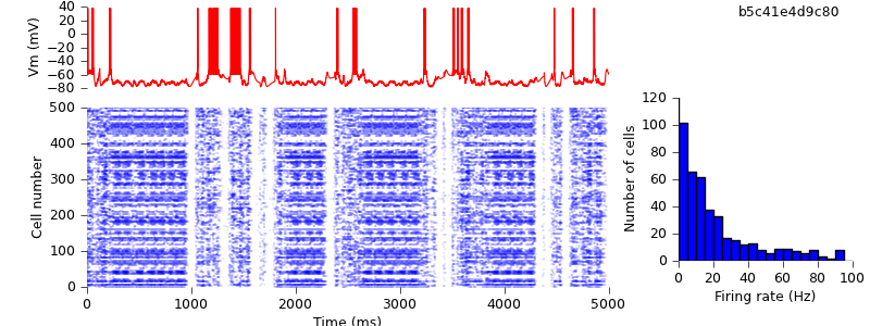
$ hg update -r 5  # refactoring of original Python conversion, putting more of the code into the cell classes.
$ python demo_cx05_N=500b_LTS.py
![]()
Replacing synapse mechanisms with ExpSyn
The multiAMPAexp and related mechanisms implement a model with an instantaneous step followed by exponential decay of the synaptic conductance. As noted above, communication between pre- and post-synaptic neurons is via pointers. The ExpSyn model used in PyNN to implement the same conductance dynamics uses NEURON's NetCon mechanism to communicate, which has the advantage that the network can be parallelized using MPI. Otherwise, the only important difference between multiAMPAexp and NetCon is that the former has a dead time of one millisecond after a conductance step in which any incoming spikes have no effect.
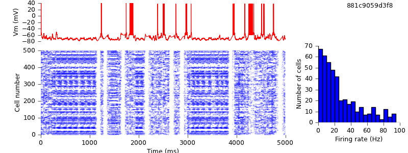
$ hg update -r 7  # replaced multiStimexp, multiAMPAexp and multiGABAAexp with ExpSyn
$ python demo_cx05_N=500b_LTS.py
$ python plot.py spiketimes_cx05_LTS500b.dat numspikes_cx05_LTS500b.dat Vm170_cx05_LTS500b.dat
![]()
Despite this difference, the models give comparable results.
Replacing input spike generation mechanism with NetSimFD
We have now replaced almost all the NMODL mechanisms from the original model with their equivalents, or near-equivalents, from PyNN. Only one remains, the gen mechanism for generating random spike trains with Poisson statistics.
The replacement with the NetStimFD mechanism from PyNN is straightforward. In fact, NetStimFD is a minor modification of Michael Hines' NetStim to have fixed duration rather than fixed number of spikes, and an interval that can safely be varied during the simulation. NetStim in turn is a modification of Destexhe and Mainen's gen to work with CVODE and NetStim.
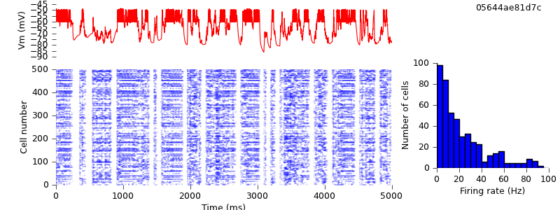
$ hg update -r 8  # replaced gen mechanism with NetStimFD
$ python demo_cx05_N=500b_LTS.py
![]()
We see that network activity dies out after a few thousand milliseconds. Changing the RNG seeds restores the persistence of the activity.
$ hg update -r 9  # changed seed for random spike generation.
$ python demo_cx05_N=500b_LTS.py
$ python plot.py spiketimes_cx05_LTS500b.dat numspikes_cx05_LTS500b.dat Vm170_cx05_LTS500b.dat
![]()

Replacing locally-defined AdExp cell class with BretteGerstnerIF from pyNN.neuron
Part 2 of our conversion strategy, replacing the original NMODL mechanisms with the nearest equivalent from PyNN, is now complete. The third and final part is to replace NEURON-specific Python code with its PyNN equivalent, starting with the cell model - instead of our own AdExp class, we use BretteGerstnerIF from the pyNN.neuron module.
$ hg update -r 10  # replaced locally-defined AdExp cell class with BretteGerstnerIF from pyNN.neuron
$ python demo_cx05_N=500b_LTS.py
$ python plot.py spiketimes_cx05_LTS500b.dat numspikes_cx05_LTS500b.dat Vm170_cx05_LTS500b.dat
![]()
As expected, the results are unchanged:
Replacing lists of cells by PyNN Populations
A small but important change, now. PyNN automatically parallelizes your code - the same script will run both on a single computer and on a cluster using MPI - but to run in parallel requires a non-zero synaptic delay. We therefore increase the synaptic delays in the model from zero to 0.1 ms.
$ hg update -r 12  # changed synaptic delays from zero to 0.1 ms
$ python demo_cx05_N=500b_LTS.py
$ python plot.py spiketimes_cx05_LTS500b.dat numspikes_cx05_LTS500b.dat Vm170_cx05_LTS500b.dat
![]()
This has quite a large quantitative effect, but qualitatively, we still see the alternation of up- and down-states.
PyNN is designed to make it easier to work with populations of neurons. Thus rather than creating cells one at a time and appending them to a list:
neuron = []
for nbactual in range(0, N_E):
    neuron.append(CXcell(**RS_parameters))
we create an entire population of neurons in one command:
neurons = pyNN.Population(N_CX, pyNN.EIF_cond_exp_isfa_ista, RS_parameters)
(note that EIF_cond_exp_isfa_ista is a PyNN "standard" cell model, which is implemented by the BretteGerstnerIF model in pyNN.neuron behind the scenes).
Similarly, recording spikes can be done with a single command:
neurons.record()
as can writing out the results to file:
neurons.printSpikes("spiketimes_%s.dat" % MODEL_ID)
$ hg update -r 13  # replaced list of cells by PyNN Population
$ python demo_cx05_N=500b_LTS.py
![]()
The PyNN output file format is slightly different to Alain's original format, so minor changes to our plotting script are needed.
$ hg update -r 14  # updated plotting script to handle PyNN output format
$ python plot.py spiketimes_cx05_LTS500b.dat numspikes_cx05_LTS500b.dat Vm_cx05_LTS500b.dat 170
As expected, the simulation output is unchanged.

Replacing direct NetCon creation with pyNN.connect()
In the next change, we replace NEURON's method of creating connections (creating NetCon objects) with the PyNN connect() method. (In fact, the implementation of connect() in pyNN.neuron does create NetCons behind the scenes, but of course the pyNN.nest implementation of the same function does not.)
The connect() function (and the more general Projection class) allows connecting entire populations at once, but here, to minimize the changes from the original script, we use it like NetCon, to connect one pair of neurons at a time. i.e. we replace:
nc = h.NetCon(neurons[j]._cell.source, neurons[i]._cell.esyn,
              neurons[j]._cell.adexp.vspike, DT, AMPA_GMAX,
              sec=neurons[j]._cell)
with:
nc = pyNN.connect(neurons[j], neurons[i], weight=AMPA_GMAX,
                  delay=DT, synapse_type="esyn")
$ hg update -r 15  # replaced list of spike sources by PyNN Population and direct NetCon creation with pyNN.connect()
$ python demo_cx05_N=500b_LTS.py
$ python plot.py spiketimes_cx05_LTS500b.dat numspikes_cx05_LTS500b.dat Vm_cx05_LTS500b.dat 170
![]()
The simulation output is unchanged.
Removing the final fragments of NEURON-specific code
We're almost there. There are just a few things more until this script can run with NEST as well as NEURON. First, we need to make use of the NEURON GUI optional.
$ hg update -r 16 # added option to run with or without GUI
![]()
Then, we replace use of Hoc's Random class with PyNN's NumpyRNG, and replace hard-coded references to pyNN.neuron with the ability to specify the simulator on the command line:
SIMULATOR = sys.argv[-1]
exec("import pyNN.%s as pyNN" % SIMULATOR)
The final change, for compatibility with the other PyNN backends, is not to explicitly represent the spikes in the recorded membrane potential: rather the membrane potential is immediately reset on passing threshold. This does not change the recorded spike times, it just changes the appearance of the membrane potential trace when plotted.
$ hg update -r 17  # script now written using purely PyNN
$ python demo_cx05_N=500b_LTS.py neuron
$ python plot.py spiketimes_cx05_LTS500b_neuron.dat numspikes_cx05_LTS500b_neuron.dat Vm_cx05_LTS500b_neuron.dat 170
![]()
Because we are using different random number generators, the simulation output is quantitatively different, but the up- and down-state pattern is preserved.
The conversion is complete. Running the same simulation with NEST requires no changes to the code, merely changing one argument on the command line:
$ python demo_cx05_N=500b_LTS.py nest
$ python plot.py spiketimes_cx05_LTS500b_nest.dat numspikes_cx05_LTS500b_nest.dat Vm_cx05_LTS500b_nest.dat 170
![]()
There is still one major source of difference between the NEST and NEURON simulations: each simulator generates its own Poisson spike trains. So that both simulations have exactly identical inputs, we need to generate the spike trains ourselves, and use SpikeSourceArray instead of SpikeSourcePoisson
$ hg update -r 18  # switched from SpikeSourcePoisson to SpikeSourceArray, so as to use the same input spike times for the different simulators
$ python demo_cx05_N=500b_LTS.py nest
$ python plot.py spiketimes_cx05_LTS500b_nest.dat numspikes_cx05_LTS500b_nest.dat Vm_cx05_LTS500b_nest.dat 170
![]()
$ python demo_cx05_N=500b_LTS.py neuron
$ python plot.py spiketimes_cx05_LTS500b_neuron.dat numspikes_cx05_LTS500b_neuron.dat Vm_cx05_LTS500b_neuron.dat 170
![]()
Of course, even now the NEURON and NEST traces are not the same, past the first few milliseconds: the high degree of recurrency of the network means that small numerical differences arising from the different implementations of the underlying equations are rapidly amplified. Nevertheless, both simulations demonstrate the same qualitative behaviour, and the length of time before divergence occurs ought to increase as the integration time step is decreased. Testing that is left as an exercise for the reader :-)