Modelling simple neurons with PyMOOSE

Tags: Python, MOOSE

7th January 2011

MOOSE (Multiscale Object-oriented Simulation Environment) is a modelling framework for biological and neuronal networks, developed in Upinder Bhalla's lab at the NCBS in Bangalore. In terms of concepts and goals, it is a descendant of the GENESIS 2 simulator (another descendant being GENESIS 3).

What I find interesting about MOOSE is the wide range of biological scales that can be modelled, from biochemical signalling pathways up to large-scale neuronal networks, and the possibility of combining these in a single, multiscale model.

MOOSE comes with a graphical interface, but what I find most interesting is its Python interface, developed by Subhasis Ray. PyMOOSE is described in an article in Frontiers in Neuroinformatics, which gives a good ideas of the capabilities of MOOSE, but does not explain how to use it. The documentation for PyMOOSE has improved rapidly of late, but is still far from comprehensive.

This post will give a brief introduction to using PyMOOSE for modelling small networks of integrate-and-fire neurons, for people who have no previous experience of using GENESIS. I made these notes for my own benefit, but they may be useful to others.

MOOSE can be downloaded from http://sourceforge.net/projects/moose/files/moose/ in various formats. I used the Debian package moose-beta-1.3.0-python26.i386.deb, which installed without problems.

Let's start by creating a single-compartment neuron:

>>> import moose
>>> soma = moose.Compartment("soma")

MOOSE uses plain SI units, so to make my life easier I'll define some scale factors:

>>> mV = 1e-3
>>> nF = 1e-9
>>> uS = 1e-6
>>> ms = 1e-3
>>> soma.initVm = -65*mV
>>> soma.Rm = 1/(0.01*uS)
>>> soma.Cm = 0.2*nF
>>> soma.Em = -65*mV

MOOSE uses different clocks to control the simulation. We will use clock 0 for integration of the differential equations and clock 1 to control initialization:

>>> ctx = moose.PyMooseBase.getContext()
>>> ctx.setClock(0, 0.025*ms, 0)
>>> ctx.setClock(1, 0.025*ms, 1)

>>> soma.useClock(0)
>>> soma.useClock(1, "init")

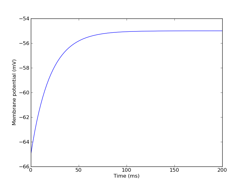
Now we have a passive compartment with no ion channels. Let's inject some current and record the membrane potential to be sure everything is working as we expect. For recording, we use a Table object:

>>> vm_table = moose.Table("Vm")
>>> vm_table.stepMode = 3
>>> vm_table.connect("inputRequest", soma, "Vm")
>>> ctx.setClock(2, 0.1*ms, 0)
>>> vm_table.useClock(2)

Note that we are recording with a larger time step than that used for integration.

Our membrane leak conductance is 0.01 µS, so an injected current of 0.1 nA should give us a depolarization of 10 mV:

>>> nA = 1e-9
>>> soma.inject = 0.1*nA

Now we run the simulation:

>>> ctx.reset()
>>> ctx.step(200*ms)

and plot the results:

>>> import numpy, pylab
>>> v = numpy.array(vm_table)/mV
>>> t = 0.1*numpy.arange(0, v.size)
>>> pylab.plot(t, v)
>>> pylab.xlabel("Time (ms)")
>>> pylab.ylabel("Membrane potential (mV)")

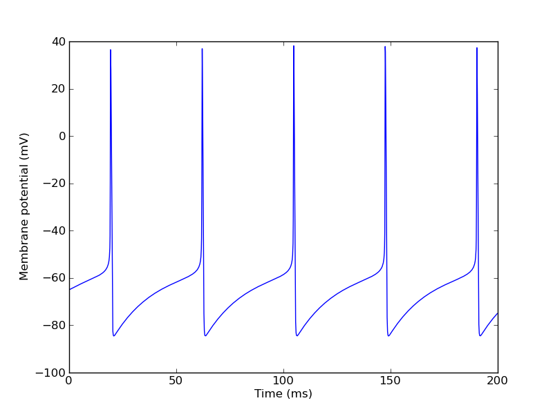
Next, we will create some ion channels:

>>> na = moose.HHChannel("na")
>>> na.Ek = 40*mV
>>> na.Gbar = 20*uS
>>> na.Xpower = 3
>>> na.Ypower = 1
>>> na.setupAlpha("X", 3.2e5 * -50*mV, -3.2e5, -1, 50*mV, -4*mV, # alpha
                      -2.8e5 * -23*mV,  2.8e5, -1, 23*mV,  5*mV) # beta
>>> na.setupAlpha("Y", 128,                 0,  0, 46*mV, 18*mV, # alpha
                       4.0e3,               0,  1, 23*mV, -5*mV) # beta

>>> k = moose.HHChannel("k")
>>> k.Ek = -90*mV
>>> k.Gbar = 6*uS
>>> k.Xpower = 4
>>> k.setupAlpha("X", 3.2e4 * -48*mV, -3.2e4, -1, 48*mV, -5*mV,
                      500,                 0,  0, 53*mV,  40*mV)

And connect them to the soma:

>>> soma.connect("channel", na, "channel")
>>> soma.connect("channel", k , "channel")

Running and plotting again:

>>> ctx.reset()
>>> ctx.step(200*ms)
>>> pylab.figure(2)
>>> pylab.plot(t, numpy.array(vm_table)/mV)
>>> pylab.xlabel("Time (ms)")
>>> pylab.ylabel("Membrane potential (mV)")

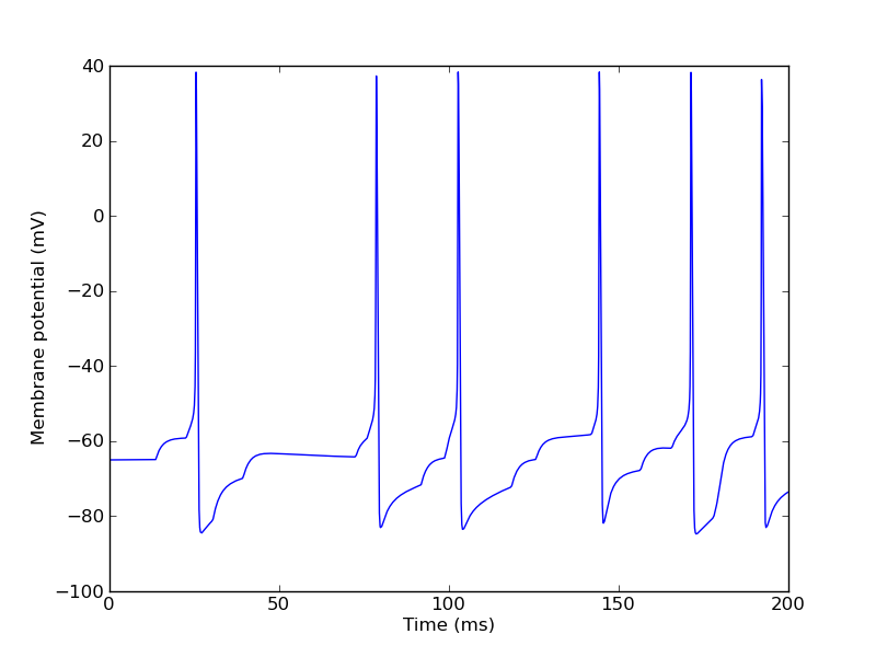
Finally, let's replace the current injection by synaptic input:

>>> soma.inject = 0
>>> synapse = moose.SynChan("excitatory")
>>> synapse.Ek = 0*mV
>>> synapse.tau1 = 0.001*ms
>>> synapse.tau2 = 2*ms
>>> synapse.Gbar = 0.01*uS
>>> soma.connect("channel", synapse, "channel")

To test the synapse we'll use a Poisson spike source:

>>> spike_source = moose.RandomSpike("input")
>>> spike_source.minAmp = 1.0
>>> spike_source.maxAmp = 1.0
>>> s = 1.0
>>> spike_source.rate = 100/s
>>> spike_source.reset = True
>>> spike_source.resetValue = 0.0

and create a synaptic connection:

>>> spike_source.connect('event', synapse, 'synapse')
>>> synapse.setWeight(0, 1.0)

As well as recording the membrane potential, we'd like to record the spike times. Again we use a Table, but this time using stepMode = 4, which detects the spikes based on threshold crossing:

>>> spike_tables = {}
>>> for label in "input", "output":
...     table = moose.Table("%s_spikes" % label)
...     table.stepMode = 4
...     table.stepSize = 1.0*mV  # threshold
...     table.useClock(0)
...     spike_tables[label] = table

>>> soma.connect('Vm', spike_tables['output'], 'inputRequest')
>>> spike_source.connect('state', spike_tables['input'], 'inputRequest')

Running the simulation:

>>> ctx.reset()
>>> ctx.step(200*ms)
>>> pylab.figure(3)
>>> pylab.plot(t, numpy.array(vm_table)/mV)
>>> pylab.xlabel("Time (ms)")
>>> pylab.ylabel("Membrane potential (mV)")

We can now print the spike times:

>>> for label in "input", "output":
...     print label, numpy.array(spike_tables[label])/ms
input [  13.6     22.575   30.425   39.35    72.55    75.825   79.075   91.775
   98.675   99.2    102.15   118.425  125.625  142.     143.675  144.45
  156.475  165.65   178.     178.925  179.75   189.5    192.925    0.   ]
output [  25.375   78.45   102.625  144.2    171.2    192.05     0.   ]

I'm not sure why there is an extraneous "0." at the end, but this can easily be discarded.

This post has only scratched the surface of MOOSE. I will post more notes as I explore further.